Classical Field Mechanics

Now, we go from just a time-dependent function like q or p to a “field” that is dependent on both temporal and spatial components:

$q(t)⟷\varphi (t,x)andp(t)⟷\Pi (t,x)$.

The field can be imagined as:

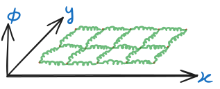
where the field points can move up & down (we neglect horizontal motion).

Lagrangian Formulation

$\dot{\varphi }=\frac{\partial \varphi }{\partial t}$

Then, we can write the action as,

$S=\int dtL(\varphi ,\dot{\varphi },\nabla \varphi ,...)$

$=\int dt(\int d^{3}xA(\varphi (x))+\int d^{3}x{d}^{3}yB(\varphi (x),\varphi (y))+...)$.

But, due to locality (the fact that it takes time for the effect to be felt) the field at $(t,0)$ does not get influenced directly and instantaneously by the field at some $(t,z)$. So, the $B$ term becomes zero. Hence, let us introduce Langrangian Density $\mathcal{L}=\mathcal{L}(\varphi ,{\partial }_{\mu }\varphi )$.

If we introduce a small deviation in the action,

$\delta S=\int dt{d}^{3}x(\delta \varphi \frac{\partial \mathcal{L}}{\partial \varphi }+\delta \dot{\varphi }\frac{\partial \mathcal{L}}{\partial \dot{\varphi }}+\delta \nabla \varphi \frac{\partial \mathcal{L}}{\partial \nabla \varphi })$

$=\int dt{d}^{3}x\delta \varphi (\frac{\partial \mathcal{L}}{\partial \varphi }-\frac{\partial }{\partial t}\frac{\partial \mathcal{L}}{\partial \dot{\varphi }}+\frac{\partial }{\partial x}\frac{\partial \mathcal{L}}{\partial {\partial }_i\varphi })+\int \delta \varphi \frac{\partial \mathcal{L}}{\partial \dot{\varphi }}{d}^{3}x+\int dt\delta \varphi \frac{\partial \mathcal{L}}{\partial {\partial }_x\varphi }{d}^{3}x+...$

Note that the second term cancels for Dirichlet boundary conditions and on assuming that $\varphi \to 0$, the third term also goes to zero.

Then, we can extract the field equations as,

$\boxed{\frac{\partial }{\partial t}\frac{\partial \mathcal{L}}{\partial \dot{\varphi }}+\frac{\partial }{\partial x^i}\frac{\partial \mathcal{L}}{\partial \frac{\partial \varphi }{\partial x^i}}-\frac{\partial \mathcal{L}}{\partial \varphi }=0}$.

We can rewrite this as

$\frac{\partial }{\partial x^{\mu }}\frac{\partial \mathcal{L}}{\partial {\partial }_x\varphi }-\frac{\partial \mathcal{L}}{\partial \varphi }=0$.

Hamiltonian Formulation

$\int d^{3}x\delta \dot{\varphi }\Pi \equiv \int d^{3}x\delta \dot{\varphi }\frac{\partial \mathcal{L}}{\delta \dot{\varphi }}$

$=\int d^{3}x\delta \dot{\varphi }(\frac{\partial \mathcal{L}}{\partial \dot{\varphi }}-\nabla \frac{\partial \mathcal{L}}{\partial \nabla \dot{\varphi }})$

such that the canonical coordinate is

$\Pi (\vec{x})=\frac{\partial \mathcal{L}}{\partial \dot{\varphi }}-\nabla \frac{\partial \mathcal{L}}{\partial \nabla \dot{\varphi }}$.

We define the Hamiltonian Density as $\mathcal{H}=\Pi .\dot{\varphi }-\mathcal{L}$.

We can now write the Hamiltonian as

$H=\int d^{3}x\mathcal{H}=\int d^{3}x(\Pi .\dot{\varphi }-\mathcal{L})$.

Now the equations of motion follow from theLegendre inverse transform such that

$\int d^{3}x\delta \varphi (\frac{\delta \mathcal{H}}{\delta \varphi })=\int d^{3}x(\frac{\delta \dot{\varphi }}{\delta \varphi }(\Pi -\frac{\delta \mathcal{L}}{\delta \dot{\varphi }})-\frac{\delta \mathcal{L}}{\delta \varphi })$.

$\dot{\varphi }=\frac{\partial \mathcal{H}}{\partial \Pi }-\nabla \frac{\partial \mathcal{H}}{\partial \nabla \Pi }\text{ and }\dot{\Pi }=-\frac{\partial \mathcal{H}}{\partial \varphi }+\nabla \frac{\partial \mathcal{H}}{\partial \nabla \varphi }$

Poisson Bracket has a generalisation,

$\frac{d}{dt}\Theta =[H,\Theta {]}_P+\frac{\partial \Theta }{\partial t}$.

• Klein-Gorden Field
• Low Energy Acoustic Phonons
• Electromagnetism
• Complex, Constrained Field